Optimization Algorithms
Optimization simply is the process of finding a solution that minimizes or maximizes an objective function while satisfying the constraints of a problem. It appears in many areas of computer science, including scheduling, routing, resource allocation, and machine learning.
While building Optinull, I implemented five optimization algorithms: Greedy, Hill Climbing (HC), Simulated Annealing (SA), Genetic Algorithms (GA), and Iterated Local Search (ILS). Each algorithm approaches the search for a good solution differently.
The important part was understanding why one algorithm improved quickly and then stopped, why another benefited from a parameter change, and why a configuration that performed well on one benchmark could be less effective on another.

The Optimization Problem
Before discussing individual algorithms, we need a way to describe the problem they are trying to solve.
Let \(S\) denote a candidate solution and let \(f(S)\) be its objective value. For a minimization problem, our goal is to find a solution \(S^*\) such that
where \(\mathcal{S}\) is the set of feasible solutions.
The objective function measures the quality of a candidate. The precise meaning of a good solution depends on the problem. In a scheduling problem, for example, we might minimize the makespan, which is the time required to complete all jobs.
For a maximization problem, the objective is reversed:
In many practical problems, the number of possible solutions is too large for exhaustive enumeration. We therefore use optimization algorithms to explore the search space and find good solutions without evaluating every possibility.
Local and global optima
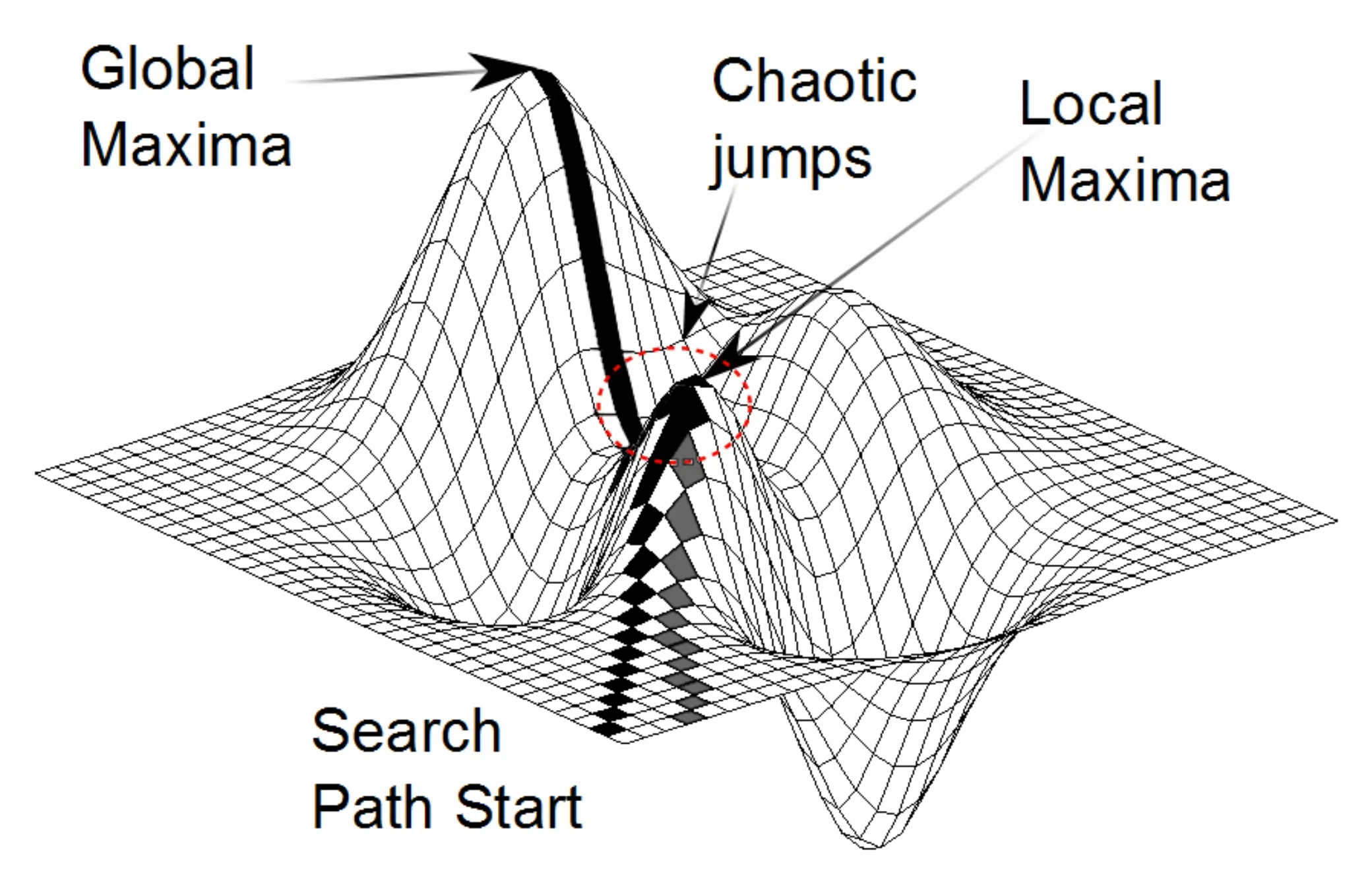
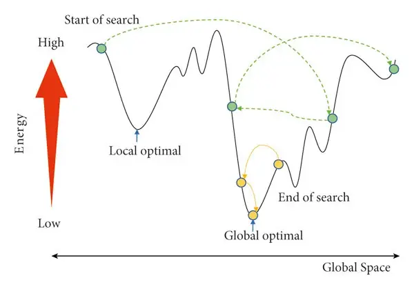
A global optimum is the best solution in the entire feasible search space. A local optimum is a solution that cannot be improved through the allowed local moves, even though a better solution might exist elsewhere.
This distinction explains why different optimization algorithms can produce different results. Some algorithms make immediate improvements, while others deliberately accept worse solutions or maintain multiple candidates to explore different regions of the search space.
The five algorithms in Optinull represent different ways of balancing these approaches.
1. Greedy Algorithm
A greedy algorithm constructs a solution by repeatedly making the locally best available choice. Instead of exploring many alternatives, it selects an action according to a heuristic and continues until a complete solution has been constructed.
The main advantage of this approach is its simplicity. A greedy algorithm can often produce a useful solution with relatively little computational effort, making it a natural starting point for more advanced optimization methods.
How the algorithm works
Suppose the current partial solution is \(S\), and let \(\mathcal{A}(S)\) be the set of actions currently available. A greedy algorithm selects the action that gives the most favorable immediate result according to its selection criterion.
where \(g(S,a)\) measures the immediate cost associated with choosing action \(a\). The action is then applied to construct the next partial solution.
The precise selection criterion depends on the problem. The important characteristic is that the algorithm makes a locally favorable choice without exhaustively comparing all possible future sequences of decisions.
General algorithm
Input: A problem instance and a greedy selection criterion.
Output: A complete solution constructed through successive local decisions.
Repeat the following steps until the solution is complete:
- Identify the available actions.
- Select the action that best satisfies the greedy criterion.
- Apply the action and update the partial solution.
The resulting solution depends heavily on the quality of the selection criterion.
Python implementation
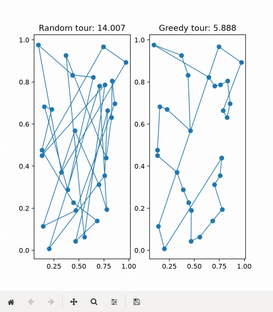
The greedy function is problem-agnostic: the actions, their costs, and how to apply them are
passed in as callables. The demo applies it to a small travelling-salesman problem (shortest closed tour
through 30 random cities), where the greedy rule becomes the nearest-neighbor heuristic. The same problem is
reused in the following sections so that the results are comparable.
Advantages and limitations
Greedy algorithms are generally easy to implement and can provide good solutions quickly. However, a locally favorable decision may restrict the choices available later, preventing the algorithm from finding a globally optimal solution.
Once an irreversible decision has been made, a basic greedy algorithm does not normally return to reconsider it. This limitation is important for problems in which early choices strongly influence later decisions.
My experience with Greedy in Optinull
Keeping Greedy as a baseline was a good decision. When a more sophisticated algorithm produces a particular objective value, the number alone does not tell us whether the additional search effort was worthwhile.
A baseline gives us a reference point. If Hill Climbing, Simulated Annealing, or a Genetic Algorithm produces a better result, we can measure the improvement over a comparatively simple method.
If the improvement is small, it gives us another question to investigate: is the problem already easy for the greedy heuristic, or are we failing to exploit the search space effectively?
2. Hill Climbing
Hill Climbing is a local search algorithm that starts with a candidate solution and attempts to improve it through small modifications. Unlike Greedy, which constructs a solution through successive choices, Hill Climbing generally begins with a complete solution and searches for a better one in its neighborhood.
The neighborhood of a solution is the set of candidates that can be reached through an allowed modification. For example, depending on the problem representation, a move might swap two elements or modify part of an existing solution.
The neighborhood function
Let \(N(S)\) denote the neighborhood of the current solution \(S\). For a minimization problem, Hill Climbing can select the best improving neighbor according to
If \(f(S')<f(S)\), the algorithm moves to \(S'\). Otherwise, if no improving neighbor exists, the search has reached a local optimum with respect to the selected neighborhood.
General algorithm
Input: An initial solution \(S\) and a neighborhood function.
Output: A locally optimal solution.
- Evaluate the current solution.
- Generate or examine neighboring solutions.
- Select an improving neighbor according to the search strategy.
- Move to the selected neighbor.
- Repeat until no acceptable improvement can be found or the evaluation budget is exhausted.
Python implementation
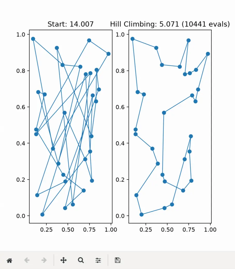
This version uses best-improvement: it examines the whole neighborhood (all pairwise swaps) and moves to the best neighbor. It also tracks the number of objective evaluations so that it can respect a budget and report how much of it was used. That count becomes important when we reuse this function inside Iterated Local Search.
The local optimum problem
The main limitation of Hill Climbing is that it does not normally accept worsening moves. Once the algorithm reaches a point where every available neighboring solution is equal or worse, it has no direct way to escape.
A local optimum does not necessarily represent a globally optimal solution. A better solution may require moving through a sequence of candidates that initially increase the objective value.
For this reason, the performance of Hill Climbing depends not only on the algorithm itself but also on the neighborhood used to explore the problem.
But Hill Climbing is still useful
Despite its limitations, Hill Climbing can be effective because it focuses its effort on immediate improvements. It also provides a local optimization procedure that can be reused by more sophisticated algorithms.
This last property became particularly relevant in Optinull when working with Iterated Local Search. Instead of treating Hill Climbing as an isolated algorithm, we can use it as the refinement step inside a larger search process.
One practical lesson was that evaluation counts need to be interpreted alongside solution quality. Hill Climbing may stop early because it has reached a local optimum, while a method that continues searching may use more evaluations and eventually find a better solution.
3. Simulated Annealing
Simulated Annealing (SA) is a probabilistic optimization algorithm inspired by the physical process of annealing. Its central idea is that accepting an occasional worsening move can help a search escape a local optimum.
Unlike basic Hill Climbing, Simulated Annealing does not reject every move that increases the objective value. Instead, it controls the probability of accepting such moves through a parameter called temperature.
Acceptance probability
Consider a minimization problem with current solution \(S\) and candidate solution \(S'\). Define the objective difference as
There are two cases.
Case 1: \(\Delta\leq0\)
The candidate is at least as good as the current solution. It can be accepted because the objective value does not increase.
Case 2: \(\Delta>0\)
The candidate is worse, but Simulated Annealing may still accept it. The probability is given by
where \(T\) is the current temperature, with \(T>0\).
A higher temperature increases the probability of accepting a worsening move. As the temperature decreases, the probability becomes smaller, and the algorithm increasingly favors improvements.
Example
Suppose a candidate solution increases the objective value by \(\Delta=5\).
At temperature \(T=10\), its acceptance probability is
The algorithm therefore accepts this worsening move with a probability of approximately \(60.65\%\).
If the temperature decreases to \(T=1\), the probability becomes
Now the same worsening move is accepted with a probability of approximately \(0.67\%\). The example illustrates how temperature changes the search behavior without changing the candidate solution or its objective difference.
Cooling schedule
The temperature decreases according to a cooling schedule. One common choice is geometric cooling:
where \(T_k\) is the current temperature and \(\alpha\) is the cooling factor.
A cooling factor close to one produces slower cooling, while a smaller factor reduces the temperature more quickly. The choice influences how much time the algorithm spends exploring through worsening moves before becoming more selective.
General algorithm
Input: An initial solution, an initial temperature, a cooling schedule, and an evaluation budget.
Output: The best solution encountered during the search.
- Initialize the current solution and record it as the best solution.
- Generate a neighboring candidate and calculate its objective difference.
- Accept an improving candidate, or accept a worsening candidate according to the temperature-dependent probability.
- Update the best solution if the new candidate improves upon it.
- Reduce the temperature according to the cooling schedule.
- Repeat until the stopping criterion is reached.
Python implementation
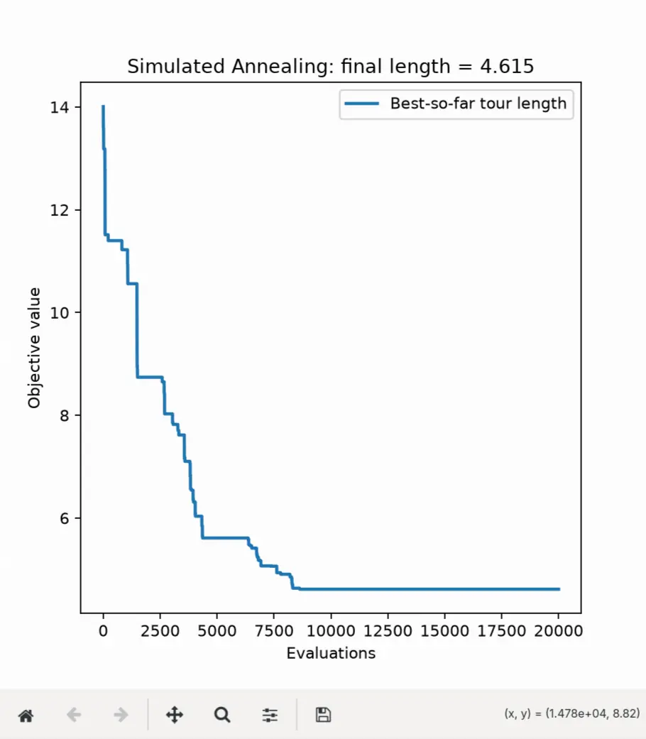
This implementation uses geometric cooling and spends one objective evaluation per iteration. It returns the best solution encountered, not the final current solution, because SA can end on a worse state than one it visited earlier. The neighbor move reverses a random segment of the tour, and the plot shows the best-so-far curve.
My experience with Simulated Annealing in Optinull
SA exposed one of the most important details of practical optimization: temperature is meaningful only in relation to the scale of the objective differences.
A temperature that works well on one problem may be inappropriate for another. If the typical worsening move increases the objective by only a small amount, a particular temperature may accept too many such moves. If typical increases are large, that same temperature may make the algorithm behave almost like Hill Climbing.
To examine this behavior, I tested temperature multipliers from \(0.05\) to \(10\) across five benchmark instances using ten random seeds.
On ft10, the best tested final-temperature configuration achieved an average objective value of
\(980.6\), compared with \(983.5\) under the automatic
settings.
The absolute improvement was
Relative to the automatic-settings mean, the improvement was approximately
This is a measurable improvement, but it is not evidence that the same configuration will perform best on every instance. Our experiments showed that the results depended on the problem being solved.
The practical lesson was that temperature parameters should not be chosen in isolation. They should be evaluated against the objective scale, the cooling schedule, and the amount of search effort available.
4. Genetic Algorithms
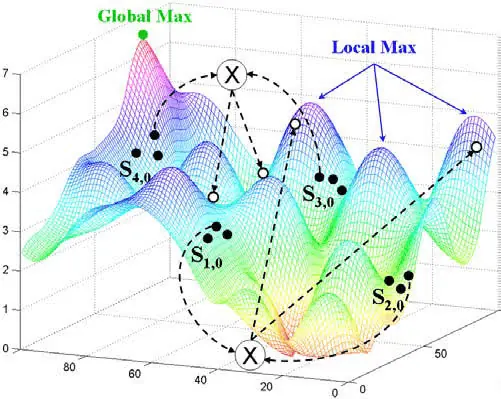
Genetic Algorithms (GAs) are population-based optimization methods inspired by biological evolution. Rather than maintaining a single candidate solution, a GA works with a population of candidates and repeatedly generates new solutions from them.
The algorithm uses selection, crossover, and mutation to evolve the population. Each operation has a different purpose: selection favors useful candidates, crossover combines information from parents, and mutation introduces variation.
Population and fitness
Let the population at generation \(t\) be
where \(m\) is the population size.
Each individual represents a candidate solution and is evaluated using the problem's objective function. The algorithm then uses a selection strategy to choose individuals for reproduction.
For a minimization problem, lower objective values represent better solutions. Depending on the implementation, the selection process may use rankings, tournaments, or a fitness transformation instead of directly treating the objective value as a fitness score.
Crossover and mutation
Crossover combines selected parent solutions to produce offspring. Its purpose is to reuse useful parts of existing solutions and potentially construct better combinations.
Mutation modifies selected parts of a candidate solution. It introduces variation into the population and can help the search discover solutions that are not easily reached through crossover alone.
Elitism is another common component. It preserves some of the best individuals so that a strong solution is not lost simply because a later generation produces worse candidates.
General algorithm
Input: A population size, selection strategy, crossover and mutation operators, and a stopping criterion.
Output: The best solution found throughout the evolutionary search.
- Generate an initial population of candidate solutions.
- Evaluate the objective value of each individual.
- Select parents according to the selection strategy.
- Apply crossover to produce offspring.
- Apply mutation to introduce variation.
- Construct the next population and preserve elite solutions when applicable.
- Repeat until the stopping criterion is reached.
Python implementation
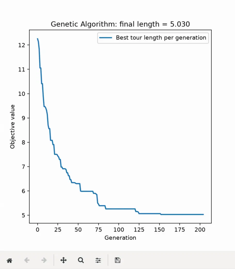
This version uses tournament selection, elitism, and an evaluation budget. The representation-specific operators (random solution, crossover, and mutation) are supplied by the caller; for the tour problem they are order crossover and a swap mutation. The mutation rate is the probability that an offspring is mutated.
Population size and evaluation budget
The population size affects how broadly the algorithm explores the search space in each generation. A larger population can maintain a wider collection of candidate solutions, but it also consumes more evaluations per generation.
At a fixed evaluation budget, there is a direct trade-off between population size and the number of generations. Increasing one generally reduces the number of opportunities available for the other.
A small population may converge quickly, but it can lose diversity and become trapped in a limited region of the search space. A large population can provide more diversity, but may not have enough generations to refine the candidates effectively.
My experience with Genetic Algorithms in Optinull
The GA experiments demonstrated that seemingly small parameter changes could improve the average objective value. However, as with SA, the results depended on the benchmark.
On ft10, a population size of \(20\) achieved an average objective value
of \(1025.5\), compared with \(1027.0\) under the automatic
settings.
We also tested a mutation rate of \(0.02\). The observed averages were:
| Benchmark | Automatic settings | Mutation rate 0.02 |
|---|---|---|
ft10 |
\(1027.0\) | \(1025.4\) |
random50 |
\(9738.9\) | \(9119.3\) |
On ft10, the difference was
On random50, the difference was substantially larger:
Because lower values are better in these minimization experiments, the mutation-rate configuration produced
better average results on both benchmarks. Relative to the automatic-settings means, the reductions were
approximately \(0.16\%\) on ft10 and \(6.36\%\)
on random50.
The difference between these improvements is the interesting part. A configuration that produces a relatively small change on one instance can produce a much more substantial change on another.
These results do not establish that a mutation rate of \(0.02\) is universally optimal. They demonstrate why parameters need to be evaluated across a range of instances instead of being selected from a single benchmark.
5. Iterated Local Search
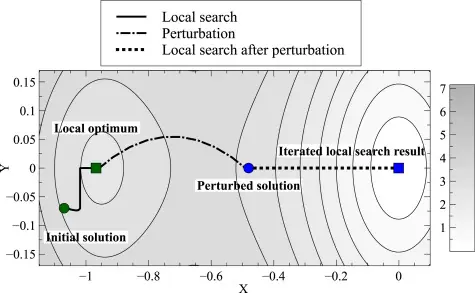
Iterated Local Search (ILS) combines local search with repeated perturbations. Its purpose is to overcome the limitation of stopping after a single local optimization process reaches a local optimum.
Instead of starting over with a completely unrelated solution every time, ILS perturbs an existing solution and applies local search again. The perturbation changes the current candidate enough to encourage exploration of a different region, while retaining the general structure of the previous solution.
Basic principle
Let \(L(S)\) denote the result of applying local search to candidate solution \(S\), and let \(P(S)\) denote a perturbation of that solution.
A simplified ILS iteration can be expressed as
After this sequence, the algorithm applies an acceptance rule to decide which solution to retain for the next iteration. The precise rule depends on the implementation and may favor the best solution, the most recent solution, or a balance between quality and exploration.
General algorithm
Input: An initial solution, a local search procedure, a perturbation operator, and a stopping criterion.
Output: The best solution found during the search.
- Generate an initial solution.
- Apply local search to obtain a locally optimized candidate.
- Perturb the candidate to explore another region of the search space.
- Apply local search to the perturbed solution.
- Evaluate the new candidate and apply the acceptance rule.
- Repeat until the evaluation budget or stopping criterion is reached.
Python implementation
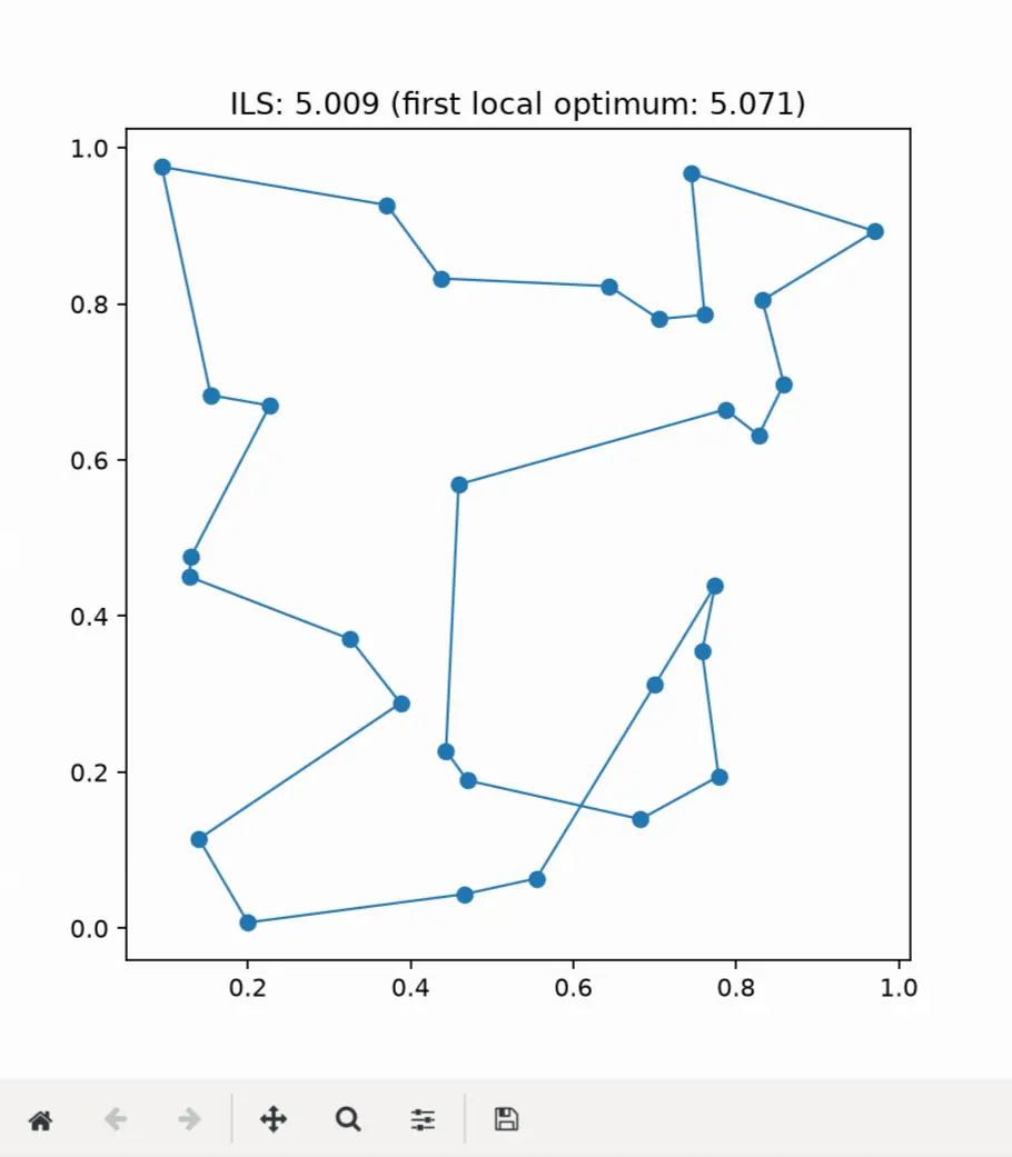
This implementation uses hill climbing (copied from section 3 so the script runs on its own) as its local search, and shares a single evaluation budget across all local search runs. The acceptance rule is simple: keep the new local optimum if it is at least as good as the current one.
The importance of perturbation strength
Perturbation strength determines how extensively the current solution is modified before local search begins again. This parameter controls the balance between exploiting a promising region and exploring a different one.
If the perturbation is too weak, local search may repeatedly return to the same local optimum. The algorithm then spends evaluations rediscovering a solution it already found.
If the perturbation is too strong, useful information from the existing solution may be lost. The resulting search can behave more like repeated random restarts than a method that systematically explores the current search landscape.
The appropriate strength depends on the representation, the neighborhood, and the structure of the problem. It must be evaluated experimentally rather than assumed to have a universally correct value.
My experience with ILS in Optinull
One implementation detail became particularly important when working with ILS: the initial local search can consume a large portion of the total evaluation budget.
For example, if the first Hill Climbing phase uses nearly the entire budget, there may be little or no room for subsequent perturbations and local searches. Changing the perturbation strength in that situation might have no measurable effect, not because the parameter is meaningless, but because the algorithm rarely reaches the part of the search that uses it.
This experience reinforced a practical debugging rule: when a parameter change appears to make no difference, inspect the execution path and budget allocation before assuming that the parameter itself is ineffective.
ILS also illustrates how algorithms can complement one another. Hill Climbing provides the local optimization step, while perturbation provides a mechanism for moving beyond the local optimum found by that step.
Rather than treating each algorithm as an isolated technique, we can therefore build more capable strategies by combining their useful components.
Comparing the Algorithms
The five algorithms differ in how they construct solutions, explore alternatives, and allocate computational effort. Their general characteristics can be summarized as follows.
| Algorithm | Main strategy | Primary limitation |
|---|---|---|
| Greedy | Make locally favorable decisions | Early decisions may prevent a globally optimal solution |
| Hill Climbing | Improve one solution through local moves | Can stop at a local optimum |
| Simulated Annealing | Accept some worsening moves according to temperature | Performance depends on calibration and the cooling schedule |
| Genetic Algorithm | Evolve a population through selection, crossover, and mutation | Can lose diversity or spend its budget inefficiently |
| Iterated Local Search | Perturb locally optimized solutions and search again | Depends on perturbation strength and budget allocation |
This comparison describes their search strategies rather than ranking their performance. No algorithm is universally best, and results depend on the particular problem, its representation, the neighborhood operators, parameter settings, and available computational resources.
Evaluating Results in Optinull
Implementing the algorithms was only one part of the work. Understanding their results required a consistent way to compare the solutions they produced.
Evaluation budget
The final objective value depends partly on how much search effort an algorithm receives. Comparing algorithms under different budgets can be misleading because a method may appear better simply because it had more opportunities to evaluate solutions.
For this reason, it is useful to compare algorithms under the same evaluation budget and examine how their best-so-far objective values change during the search.
For example, Optinull can be used to compare the results on
ft10 under two different iteration
settings:
If the ranking changes between these settings, the result suggests that the algorithms respond differently to additional search effort. An algorithm that improves quickly may be preferable under a strict budget, while another may benefit more from a longer search.
The precise interpretation of a budget should follow the implementation: iteration counts and objective evaluations are not necessarily identical, especially when an iteration evaluates multiple candidate solutions.
Repeated experiments
Stochastic algorithms can produce different results on different runs. A single execution therefore cannot fully describe their expected performance.
In our parameter experiments, we used ten random seeds across five benchmark instances. Repeated runs make it possible to compare average performance and reduce the risk of drawing conclusions from an unusually favorable or unfavorable run.
Ten seeds are a useful starting point, although additional repetitions may be necessary when results vary substantially or when small differences are important.
Optimality gap
When the optimal objective value is known, we can measure how far an obtained solution is from the optimum. For a minimization problem, the relative optimality gap is
where \(f(S)\) is the objective value of the obtained solution and \(f^*\) is the optimal objective value.
A gap of zero percent means that the solution reaches the known optimum. A positive gap indicates that its objective value is above the optimum.
Our observed benchmark results
During development, the job-shop scheduling benchmarks ft06 and ft10 provided
useful reference points because their optimal makespan values are known.
| Benchmark | Known optimum | Observed objective | Gap |
|---|---|---|---|
ft06 |
\(55\) | \(55\) | \(0\%\) |
ft10 |
\(930\) | \(983.5\) | \(5.75\%\) |
On ft06, Optinull reached the known optimum of
\(55\), resulting in a
zero-percent gap. On ft10, an objective value of \(983.5\) corresponds to
a gap of approximately \(5.75\%\) above its optimum of \(930\).
The SA experiments produced a mean of \(980.6\) for the best tested final-temperature
configuration on ft10, compared with \(983.5\) for the automatic
settings. This corresponds to a reduction in the mean objective value, but the remaining gap shows that
improving a result and reaching the optimum are two different goals.
These figures also need to be interpreted in their experimental context. The SA and GA values above compare configurations within their respective tests; they should not be treated as a definitive head-to-head ranking unless the algorithms were evaluated under matching conditions.